![]()
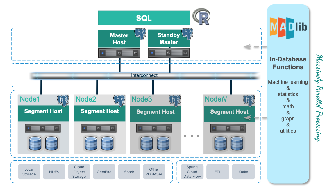
Greenplum Architecture
The main reason behind adaptation of massively parallel processing(MPP), data warehouse(DWH) solution is MPP architectural principles. These principles aim at removing main drawbacks of traditional DWH, and make MPP databases so powerful for large datasets and analytical queries.
- Shared Nothing
- Data Sharding
- Data Replication
- Distributed Transactions
- Parallel Processing
Sharding is a type of database partitioning that separates very large databases into smaller, faster, more easily managed parts called data shards. The word shard means a small part of a whole.
Database replication is the frequent electronic copying of data from a database in one computer or server to a database in another so that all users share the same level of information. The result is a distributed database in which users can access data relevant to their tasks without interfering with the work of others.
Why Do we Need MPP data Warehouse ?
First, we need to understand how to make best use of MPP data warehouse architecture. For example, MPP data warehouse works well for:-
- Relational data
- Batch processing
- Ad hoc analytical SQL
- Low concurrency
- Applications requiring ANSI SQL
MPP data warehouse solution is not the best choice for :-
- Non-relational data
- OLTP and event stream processing
- High concurrency as in OLTP
- 100+ server clusters
- Non-analytical use cases
- Geo-Distributed use cases
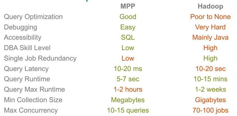
Hadoop is Popular, Why Should we choose Greenplum MPP ?
How would you choose between MPP and Hadoop based solution for your analytical workload ?
If you chose Greenplum Data Compute Appliance (aka EMC hardware) then here’s an overview of the hardware architecture and performance. You can build/acquire third party hardware for Greenplum as well. Main advantage of Greenplum DCA appliances is of course performance, technical support and timely updates/fixes.

What is Greenplum Instance
A Greenplum instance is a Greenplum application setup, which can manage one or more databases. It is hoped that in future, Greenplum will support seamless access to multiple databases as well. Similar tools are available in OLTP, and there is no reason why these should not available in DWH. Since GP DB is open source, this is also an opportunity for future development for the open source community.
Greenplum Instance is a Greenplum database system called an instance. It is possible to have more than one instance installed. A Greenplum instance can manage multiple databases. A client can connect to only one database at a time, it is not possible to query across databases.
Greenplum Schema
Schema’s are very important for meeting multiple business needs of the clients. For example, you have multiple separate business areas with their own data warehouse models and totally separate business requirements. For example, we can have prepaid and credit solutions. Similarly, we may have a separate schema for fraud analysis which is an independent service or solution. There are multiple other services for which you may need a separate schema. Great advantage of schema is you can easily query across different schemas.
Database Schema is a named container for a set of database objects, including tables, data types and functions. A database can have multiple schemas. Objects within the schema are referenced by prefixing the object name with the schema name, separated with a period.
For example, the person table in the employee schema is written as employee.person; it is the same table name that can exist in different schemas. A single query can access queries in different schemas.
Greenplum Database performs best with a denormalized schema design suited for MPP analytical processing, a star or snowflake schema, with large centralized fact tables connected to multiple smaller dimension tables.

Storage and Orientation
Use heap storage for tables and partitions that will receive iterative batch and singleton UPDATE, DELETE, and INSERT operations.
Use heap storage for tables and partitions that will receive concurrent UPDATE, DELETE, and INSERT operations.
- Never perform singleton INSERT, UPDATE, or DELETE operations on append-optimized tables.
- Never perform concurrent batch UPDATE or DELETE operations on append-optimized tables.
- Concurrent batch INSERT operations are okay.
Use append-optimized storage for tables and partitions that are updated infrequently after the initial load and have subsequent inserts only performed in large batch operations.
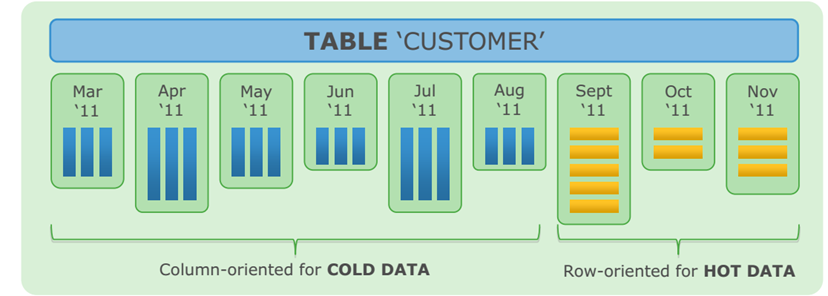
Row versus Column Oriented Storage
Use row-oriented storage for workloads with iterative transactions where updates are required and frequent inserts are performed. Use row-oriented storage when selected against the table are wide. Use row-oriented storage for general purpose or mixed workloads.
Use column-oriented storage where selects are narrow and aggregations of data are computed over a small number of columns. Use column-oriented storage for tables that have single columns that are regularly updated without modifying other columns in the row.
Understanding and Making Best Use of Polymorphic Storage
Greenplum storage types can be mixed within a table or database. It has four table types: heap, row-oriented append optimized(AO), column-oriented append optimized(AO), and external.
Data Distributions
In Greenplum Database, the segments are where data is stored and where most query processing occurs. User-defined tables and their indexes are distributed across the available segments in the Greenplum Database system; each segment contains a distinct portion of the data. Segment instances are the database server processes that serve segments. Users do not interact directly with the segments in a Greenplum Database system, but do so through the master.
In the reference Greenplum Database hardware configurations, the number of segment instances per segment host is determined by the number of effective CPUs or CPU cores.
For example, if your segment hosts have two dual-core processors, you may have two or four primary segments per host. If your segment hosts have three quad-core processors, you may have three, six or twelve segments per host. Performance testing will help decide the best number of segments for a chosen hardware platform.
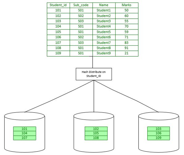
The primary strategy and goal is to spread data evenly across as many nodes (and disks) as possible :-

Figure : Data distribution across many nodes
Create Table | Defining Data Distribution
We use Create Table to define data distribution method. Every table has a distribution method
DISTRIBUTED BY (column) clause which uses a hash distribution.
We can also use DISTRIBUTED RANDOMLY clause which uses a random distribution which is not guaranteed to provide a perfectly even distribution.
CREATE TABLE tablename (
Col1 data_type,
Col2 data_type,
Col3 data_type …)
[DISTRIBUTE BY (column_name)] — Used for Hash distribution
[DISTRIBUTED RANDOMLY] — Used for Random distribution, distributes on round robin fashion
Here is a create table example, which is using hash distribution :
=> CREATE TABLE products
(name varchar(40), prod_id integer, supplier_id integer)
DISTRIBUTED BY (prod_id);
For large tables significant performance gains can be obtained with local joins (co-located joins).
Distribute on the same column for tables commonly joined together in WHERE clause. Join is performed within the segment. Each segment operates independently of other segments.
Hash distribution typically eliminates or minimizes motion operations such as broadcast motion and redistribute motion.
Create Table using Random Distribution
Random distribution clause uses a random algorithm. It distributes data across all segments. There can be minimal data skew but not guaranteed to have a perfectly even distribution. Any query that joins to a table that is distributed randomly will require a motion operation
- Redistribute motion
- Broadcast motion
Redistribute Motions: In order to perform a local join, rows must be located together on the same segment and in case if absence of which, a dynamic redistribution of the needed rows from one of the segment instance to another segment instance will be performed. This operation might be quite expensive in case of large fact tables.
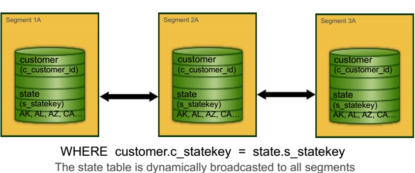
Broadcast Motions: In the broadcast motion, every segment will sends the copy of table to all segment instances. Optimizer always picks only small table for broadcast motions.
Changing Data Distribution
You can use the ALTER TABLE command to change the distribution policy for a table. For partitioned tables, changes to the distribution policy recursively apply to the child partitions.
This operation preserves the ownership and all other attributes of the table.
For example, the following command redistributes the table sales across all segments using the customer_id column as the distribution key:
>> ALTER TABLE sales SET DISTRIBUTED BY (customer_id);
When you change the hash distribution of a table, table data is automatically redistributed.
However, changing the distribution policy to a random distribution will not cause the data to be redistributed.
For example:
>> ALTER TABLE sales SET DISTRIBUTED RANDOMLY;
When you change the hash distribution of a table, table data is automatically redistributed.
However, changing the distribution policy to a random distribution will not cause the data to be redistributed.
For example:
>> ALTER TABLE sales SET DISTRIBUTED RANDOMLY;
Redistributing Table Data
To redistribute table data for tables with a random distribution policy (or when the hash distribution policy has not changed) use REORGANIZE=TRUE.
This sometimes may be necessary to correct a data skew problem, or when new segment resources have been added to the system.
For example:
>> ALTER TABLE sales SET WITH (REORGANIZE=TRUE);
Data Distribution Best Practices
- Use the Same Distribution Key for Commonly Joined Tables.
- Distribute on the same key used in the join (WHERE clause) to obtain local joins
- Commonly Joined Tables should use the Same Data Type for Distribution Keys
- Values with different data types might appear the same but they HASH to different values
- Resulting in like rows being stored on different segments
- Requiring a redistribution before the tables can be joined

Partitioning
For a typical data warehouse, you are dealing with very large datasets. You are also dealing with specific analysis patterns that are frequently repeated. Using partitioning; a table is divided into smaller child files using a range or a list value, such as a date range or a country code.
Partitioning a table can improve query performance and simplify data administration. When a query predicate filters on the same criteria used to define partitions, the optimizer can avoid searching partitions that do not contain relevant data.
A common application for partitioning is to maintain a rolling window of data based on date. For example, a fact table containing the most recent 12 months of data. Using the ALTER TABLE statement, an existing partition can be dropped by removing its child file. This is much more efficient than scanning the entire table and removing rows with a DELETE statement.
Partitions may also be subpartitioned. For example, a table could be partitioned by month, and the month partitions could be subpartitioned by week. Greenplum database creates child files for the months and weeks.
The actual data, however, is stored in the child files created for the week subpartitions—only child files at the leaf level hold data.
Defining Partitioning
We use the Create Table statement to define the partitioning strategy for the table. It reduces the amount of data to be scanned by reading only the relevant data needed to satisfy a query. The goal is to achieve partition elimination.
Greenplum database supports range and list partitioning schemes:
- Range Partitioning: Division of data based on a numerical range, such as date or price.
- List Partitioning: Division of data based on a list of values, such as sales territory or product line.
- A combination of both types.
Partitioning also uses table inheritance and constraints; while establishing a persistent relationship between parent and child tables.
Partitioning Guidelines
- It uses table partitioning on large tables to improve query performance
- Table partitioning is not a substitute for distributions
- Use if the table can be divided into rather equal parts based on a
defining criteria - For example, range partitioning on date
- No overlapping ranges or duplicate values
- And the defining partitioning criteria is the same access pattern used in query predicates
– WHERE date = ‘1/30/2012’
Defining Range Partitions
A date range partitioned table uses a single date or timestamp column as the partition key column. You can use the same partition key column to further sub-partition a table if necessary (for example, to partition by month and then sub-partition by day).
When date partitioning a table, consider partitioning by the most granular level you are interested in. For example, partition by day and have 365 daily partitions, rather than partition by year then sub-partition by month then sub-partition by day.
A multi-level design can reduce query planning time, but a flat partition design will execute faster at query run time. You can have Greenplum Database automatically generate partitions by giving a START value, an END value, and an EVERY clause that defines the partition increment value. By default, START values are always inclusive and END values are always exclusive.
For example:
CREATE TABLE sales (id int, date date, amt decimal(10,2))
DISTRIBUTED BY (id)
PARTITION BY RANGE (date)
( START (date ‘2008-01-01’) INCLUSIVE
END (date ‘2009-01-01’) EXCLUSIVE
EVERY (INTERVAL ‘1 day’) );
You can also declare and name each partition individually. For example:
CREATE TABLE sales (id int, date date, amt decimal(10,2))
DISTRIBUTED BY (id)
PARTITION BY RANGE (date)
( PARTITION Jan08 START (date ‘2008-01-01’) INCLUSIVE ,
PARTITION Feb08 START (date ‘2008-02-01’) INCLUSIVE ,
PARTITION Mar08 START (date ‘2008-03-01’) INCLUSIVE ,
PARTITION Apr08 START (date ‘2008-04-01’) INCLUSIVE ,
PARTITION May08 START (date ‘2008-05-01’) INCLUSIVE ,
PARTITION Jun08 START (date ‘2008-06-01’) INCLUSIVE ,
PARTITION Jul08 START (date ‘2008-07-01’) INCLUSIVE ,
PARTITION Aug08 START (date ‘2008-08-01’) INCLUSIVE ,
PARTITION Sep08 START (date ‘2008-09-01’) INCLUSIVE ,
PARTITION Oct08 START (date ‘2008-10-01’) INCLUSIVE ,
PARTITION Nov08 START (date ‘2008-11-01’) INCLUSIVE ,
PARTITION Dec08 START (date ‘2008-12-01’) INCLUSIVE
END (date ‘2009-01-01’) EXCLUSIVE );
A numeric range partitioned table uses a single numeric data type column as the partition key column. For example:
CREATE TABLE rank (id int, rank int, year int, gender char(1), count int)
DISTRIBUTED BY (id)
PARTITION BY RANGE (year)
( START (2001) END (2008) EVERY (1),
DEFAULT PARTITION extra );
A list partitioned table can use any data type column that allows equality comparisons as its partition key column. A list partition can also have a multi-column (composite) partition key, whereas a range partition only allows a single column as the partition key.
For list partitions, you must declare a partition specification for every partition (list value) you want to create. For example:
CREATE TABLE rank (id int, rank int, year int, gender char(1), count int )
DISTRIBUTED BY (id)
PARTITION BY LIST (gender)
( PARTITION girls VALUES (‘F’),
PARTITION boys VALUES (‘M’),
DEFAULT PARTITION other );
Here’s another example : –
CREATE TABLE bar (bid integer, bloodtype text, bdate date)
DISTRIBUTED by (bid)
PARTITION BY LIST(bloodtype)
(PARTITION a values(‘A+’, ‘A’, ‘A-‘),
PARTITION b values (‘B+’, ‘B-‘, ‘B’),
PARTITION ab values (‘AB+’, ‘AB-‘, ‘AB’),
PARTITION o values (‘O+’, ‘O-‘, ‘O’)
DEFAULT PARTITION unknown);
Altering a Partition with Alter Table
You can add a partition to a partition design with the ALTER TABLE command. If the original partition design included sub-partitions defined by a sub-partition template, the newly added partition is sub-partitioned according to that template.
For example:
ALTER TABLE sales ADD PARTITION
START (date ‘2009-02-01’) INCLUSIVE
END (date ‘2009-03-01’) EXCLUSIVE;
Compression
When doing analytics with large data sets, queries often read the entire table from disk. If the table is compressed, the smaller size can result in many fewer disk reads, enhancing query performance.
Small tables need not be compressed because it will yield neither significant performance gain nor storage gains. Compression and expansion require CPU resources. We use compression on large append-optimized and partitioned tables to improve I/O across the system. With compression, we can balance higher levels of compression with the time and CPU cycles needed to compress and uncompress data.
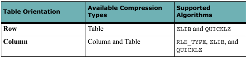
Rich compression functionality, definable column by column:
- Block compression: Gzip (levels 1-9), QuickLZ
- Stream compression: RLE (levels 1-4)
Like distribution, you specify compression when you create a table.
CREATE TABLE foobar (fid INT, ft TEXT)
WITH (compresstype = quicklz, orientation=column, appendonly=true)
DISTRIBUTED by (fid);
A column-oriented table also can have different compression strategies for different columns.
create table comp1
( cid int ENCODING(compresstype=quicklz),
ct text ENCODING(compresstype=zlib, compresslevel = 5),
cd date ENCODING(compresstype=rle_type),
cx smallint)
with (appendonly=true, orientation=column)
distributed by (cid);
QuickLZ compression generally uses less CPU capacity and compresses data faster at a lower compression ratio than zlib. zlib provides higher compression ratios at lower speeds. At compression level 1 (compresslevel=1), QuickLZ and zlib have comparable compression ratios, though at different speeds. Using zlib with compresslevel=6 can significantly increase the compression ratio compared to QuickLZ, though with lower compression speed.
Data Loading in Greenplum
There are two major approaches for data loading in Greenplum i.e. bulk data loading and incremental data loading. In Greenplum, we can use different commands for incremental and bulk data loading as seen here.

External Tables
External table feature allows you to access external files as if they were regular database tables. It is used with gpfdist to provide full parallelism to load or unload data.
It supports querying using SQL. You can also create views for external tables.
Using this feature, you can create readable external tables for loading data, while having power to perform common ETL tasks.
You can also create writeable external tables for unloading data. In this case, you will select data from database table to insert into writeable external table. This involves sending data to a data stream.
File Based External Tables
File based external tables are used to specify format of input files using FORMAT clause.
Specify location of external data sources (URIs).
Specify protocol to access external data sources i.e. gpfdist and gpfdists.
gpfdist provides the best performance. In this case segments access external files in parallel up to the value of gp_external_max_segments (Default 64).
gpfdists is a secure version of gpfdist. file:// segments access external files in parallel based on the number of URIs.
Data Load Using Regular External Tables
Create external table is a metadata operation for setting up external file linking with data files.
No data is actually moved here.
File based (flat files)
– gpfdist provides the best performance
=# CREATE EXTERNAL TABLE ext_expenses (name text,
date date, amount float4, category text, description text)
LOCATION
( ‘gpfdist://etlhost:8081/*.txt’, ‘gpfdst://etlhost:8082/*.txt’)
FORMAT ’TEXT’ (DELIMITER ‘|’ );
Here’s how we set up the gpfdist processes:
$ gpfdist –d /var/load_files1/expenses –p 8081 –l /home/gpadmin/log1 &
$ gpfdist –d /var/load_files2/expenses –p 8082 –l /home/gpadmin/log2 &
COPY
It is quick and easy method that recommended for small data loads. Copy is not recommended for bulk loads.
It can be used to load data from file or standard input. It is not parallel because it uses a single process run on the master.
You can improve data loading performance by running multiple COPY commands concurrently. In such a case, data must be divided across all concurrent processes. Source file must be accessible by the master.
Example :
>> COPY my_table FROM ‘c:\downloads\file.csv’ DELIMITERS ‘,’ CSV QUOTE ””;
GPLOAD Utility
GPLOAD utility provides an interface to readable external tables. It invokes gpfdist for parallel loading. It creates an external table based on source data defined.
It uses load specification defined in a YAML formatted control file:
- INPUT
Hosts, ports, file structure
- OUTPUT
▪ Target Table
▪ MODES: INSERT, UPDATE, MERGE
▪ BEFORE & AFTER SQL statements
Greenplum Data Loading Performance
Greenplum has Industry leading data loading performance at 10+TB per-hour per-rack. Its
Scatter-Gather Streaming™ provides true linear scaling. It has support for both large-batch and continuous real-time loading strategies. Greenplum enables complex data transformations using in-flight transparent interfaces to loading via support files, application, and services.

Data Warehouse Optimization
Data warehouse best practices for performance include:
- Data Distribution
- Partitioning
- Storage Orientation
- Compression
- Data Loading
Data Type and Byte Alignment
For ensuring optimal performance, the optimal layout for columns in heap tables is as follows:
– 8 byte first (bigint, timestamp)
– 4 byte next (int, date)
– 2 byte last (smallint)
Put distribution and partition columns up front
– Two 4 byte columns = an 8 byte column
Analyzing Database Statistics
After a load you should analyze the tables, using the ANALYZE command. This gathers statistics on the data distribution, which the optimizer uses to choose an explain plan.
Unanalyzed tables lead to less than optimal explain plans and less than optimal query
performance. Updated statistics are critical for the Query Planner to generate optimal query plans. When a table is analyzed table information about the data is stored into system catalog tables
Always run ANALYZE after loading data. Run ANALYZE after INSERT, UPDATE and DELETE operations that significantly changes the underlying data. For very large tables it may not be feasible to run ANALYZE on the entire table.
ANALYZE may be performed for specific columns
Run ANALYZE for :
- Columns used in a JOIN condition
- Columns used in a WHERE clause
- Columns used in a SORT clause
- Columns used in a GROUP BY or HAVING Clause
VACCUM
VACUUM reclaims physical space on disk from deleted or updated rows or aborted load/insert operations. VACUUM collects table-level statistics such as the number of rows and pages.
- Run VACUUM after
- Large DELETE operations
- Large UPDATE operations
- Failed load operations
Parallel Query Optimization
Cost-based optimization looks for the most efficient plan. Physical plan contains
scans, joins, sorts, aggregations, etc. Global planning avoids sub-optimal ‘SQL pushing’ to segments. Directly inserts ‘motion’ nodes for inter-segment communication.

Greenplum Commands
Enter these commands to start/stop or check the status of Greenplum database:
| Command | Explanation |
| $ gpstate | Display status of master and segment processes |
| $ gpstop | Display parameters for master and segment processes that are to be stopped, and allows you to stop Greenplum instance |
| $ gpstart | Display parameters for master and segment processes that are to be started, and allows you to start Greenplum instance |
PSQL Commands
| Command | Purpose |
| \g [file] or ; | Execute query and send result to file or query |
| \q | Quit psql |
| \e [FILE] | Edit the query buffer |
| \r | Reset the query buffer |
| \s [FILE] | Display history, save to file |
| \w FILE | Display history, or save to file |
| \i FILE | Execute command from file |
| \d | List tables, views and sequences |
| \d+ NAME | Describe table, view, sequence, or index |
| \cd [DIR} | Change the current working directory |
| \timing [on|off] | Toggling timing of commands |
| \c[onnect] [DBNAME…..] | Connect to new database |
Essential Database Administration
Connect to the tutorial database as gpadmin.
$ psql -U gpadmin tutorial
Creating Database
To use the CREATE DATABASE command, you must be connected to a database. With a newly installed Greenplum Database system, you can connect to the template1 database to create your first user database.
The createdb utility, entered at a shell prompt, is a wrapper around the CREATE DATABASE command.
To list all the existing databases, we use:
$ psql –l
To drop an existing database:
$ dropdb tutorial
Creating a new database using createdb utility:
$ createdb tutorial
Creating Schema
Here we are using faa tutorial in getting started guide for Greenplum. First of all connect with tutorial database, where we want to create schema.
Drop faa schema if it already exists :-
DROP SCHEMA IF EXISTS faa CASCADE
Create new schema named faa :-
=# CREATE SCHEMA faa;
Add the faa schema to the search path:
=# SET SEARCH_PATH TO faa, public, pg_catalog, gp_toolkit;
View the search path:
=# SHOW search_path;
Creating Column Oriented Table
Create a column-oriented version of the FAA On Time Performance fact table and insert the data from the row-oriented version.
=# CREATE TABLE FAA.OTP_C (LIKE faa.otp_r)
WITH (appendonly=true, orientation=column)
DISTRIBUTED BY (UniqueCarrier, FlightNum)
PARTITION BY RANGE(FlightDate)
( PARTITION mth
START(‘2009-06-01’::date)
END (‘2010-10-31’::date)
EVERY (‘1 mon’::interval)\d
);
=# INSERT INTO faa.otp_c
SELECT * FROM faa.otp_r;
Comparing Table Sizes for Row vs Column Orientation
=# SELECT
pg_size_pretty(pg_total_relation_size(‘faa.otp_r’));
pg_size_pretty
—————-
383 MB
(1 row)
=# SELECT pg_size_pretty(pg_relation_size(‘faa.otp_c’));
pg_size_pretty
—————-
0 bytes
(1 row)
=# SELECT
pg_size_pretty(pg_total_relation_size(‘faa.otp_c’));
pg_size_pretty
—————-
256 kB
(1 row)
Checking Data Distribution on Segments
One of the goals of distribution is to ensure that there is approximately the same amount of data in each segment. The query below shows one way of determining this.
=# SELECT gp_segment_id, COUNT(*) FROM faa.otp_c
GROUP BY gp_segment_id
ORDER BY gp_segment_id;
Greenplum Getting Started Exercise
Login as GP Admin
$ gpadmin
Password is pivotal
Start the Greenplum Database
$./start_all.sh
To check the current status of the Greenplum Database instance:
1. Run the gpstate command:
$ gpstate
The command displays the status of the master and segment processes. If the
Greenplum system is not running, the command displays an error message.
Shut down the Greenplum Database instance
1. Run the gpstop command:
$ gpstop
Displays parameters for the master and segment processes that are to be stopped.
2. Enter y when prompted to stop the Greenplum instance.
To start the Greenplum Database instance:
1. Run the gpstart command:
$ gpstart
The command displays parameters for the master and segment processes that are
to be started.
2. Enter y when prompted to continue starting up the instance.
When newly installed, a Greenplum Database instance has three databases:
• The template1 database is the default template used to create new databases. If
you have objects that should exist in every database managed by your Greenplum
Database instance, you can create them in the template1 database.
• The postgreSQL and template0 databases are used internally and should not be
modified or dropped. If you have modified the template1 database you can use
the template0 database to create a new database without your modifications.
Connect to a database with psql
The psql command is an interactive, command-line client used to access a
Greenplum database.
Since there is no gpadmin database by default, you must at least
specify the database name on the psql command line.
To connect to a database with default connection parameters:
$ psql template1
To specify connection parameters on the command line:
$ psql -h localhost -p 5432 -U gpadmin template1
To set connection parameters in the environment:
$ export PGPORT=5432
$ export PGHOST=localhost
$ export PGDATABASE=template1
$ psql
PSQL Meta Commands
In addition to SQL statements, you can enter psql meta-commands, which begin with a backslash (\). Here are some common psql meta-commands:
• Enter \g instead of a semicolon to terminate a SQL statement
• Enter \e to edit the buffer in an external editor (vi by default)
• Enter \p to display the contents of the query buffer
• Enter \r to reset the query buffer, abandoning what you have entered
• Enter \l to list databases
• Enter \d to list tables, views, and sequences
• Enter \q to exit psql
• Enter \h to display help for SQL statements
• Enter \? to display help for psql
○ When using the psql command line, you may list all schema with command \dn
Putty Based Login for Greenplum VM
Setup ssh connection with localhost using putty for accessing greenplum localhost. This would greatly ease development in the local environment.
To show tables Using SQL:-
>> SELECT * FROM pg_catalog.pg_tables;
Getting Tables for your desired schema
>> SELECT * FROM pg_catalog.pg_tables where schemaname=’faa’;
Getting Fixed Number of Records from Table
>> select * from faa.otp_r limit 10;
Creating a new schema
>> create schema faa2;
Comparing Table Sizes for Row vs Column Orientation
=# SELECT
pg_size_pretty(pg_total_relation_size(‘faa.otp_r’));
pg_size_pretty
—————-
383 MB
(1 row)
=# SELECT pg_size_pretty(pg_relation_size(‘faa.otp_c’));
pg_size_pretty
—————-
0 bytes
(1 row)
=# SELECT
pg_size_pretty(pg_total_relation_size(‘faa.otp_c’));
pg_size_pretty
—————-
256 kB
(1 row)
Checking Data Distribution on Segments
SELECT gp_segment_id, COUNT(*) FROM faa.otp_c
GROUP BY gp_segment_id
ORDER BY gp_segment_id;
Range Partitioning
CREATE TABLE sales (id int, date date, amt decimal(10,2))
DISTRIBUTED BY (id)
PARTITION BY RANGE (date)
( START (date ‘2008-01-01’) INCLUSIVE
END (date ‘2009-01-01’) EXCLUSIVE
EVERY (INTERVAL ‘1 day’) );
Partitioning an Existing Table
It is not possible to partition a table that has already been created. Tables can only be partitioned at CREATE TABLE time. If you have an existing table that you want to partition, you must recreate the table as a partitioned table, reload the data into the newly partitioned table, drop the original table and rename the partitioned table to the original name. You must also regrant any table permissions. For example:
CREATE TABLE sales2 (LIKE sales)
PARTITION BY RANGE (date)
( START (date ‘2008-01-01’) INCLUSIVE
END (date ‘2009-01-01’) EXCLUSIVE
EVERY (INTERVAL ‘1 month’) );
INSERT INTO sales2 SELECT * FROM sales;
DROP TABLE sales;
ALTER TABLE sales2 RENAME TO sales;
GRANT ALL PRIVILEGES ON sales TO admin;
GRANT SELECT ON sales TO guest;
Viewing Your Partition Design
You can look up information about your partition design using the pg_partitions view. For example, to see the partition design of the sales table:
SELECT partitionboundary, partitiontablename, partitionname,
partitionlevel, partitionrank
FROM pg_partitions
WHERE tablename=’sales’;
The following table and views show information about partitioned tables.
• pg_partition – Tracks partitioned tables and their inheritance level relationships.
• pg_partition_templates – Shows the subpartitions created using a subpartition template.
• pg_partition_columns – Shows the partition key columns used in a partition design.
Compression Example
CREATE TABLE foobar (fid INT, ft TEXT)
WITH (compresstype = quicklz, orientation=column, appendonly=true)
DISTRIBUTED by (fid);